Fine-grained Urban Flow Prediction (WWW'21)

https://zhangjunbo.org/pdf/2021_WWW_UrbanFlow.pdf

Urban flow prediction benefits smart cities in many aspects, such as traffic management and risk assessment. However, a critical prerequisite for these benefits is having fine-grained knowledge of the city. Thus, unlike previous works that are limited to coarse-grained data, we extend the horizon of urban flow prediction to fine granularity which raises specific challenges: 1) the predominance of inter-grid transitions observed in fine-grained data makes it more complicated to capture the spatial dependencies among grid cells at a global scale; 2) it is very challenging to learn the impact of external factors (e.g., weather) on a large number of grid cells separately.

    To address these two challenges, we present a Spatio-Temporal Relation Network (STRN) to predict fine-grained urban flows.

• First, a backbone network is used to learn high-level representations for each cell.
• Second, we present a Global Relation Module (GloNet) that captures global spatial dependencies much more efficiently compared to existing methods.
• Third, we design a Meta Learner that takes external factors and land functions (e.g., POI density) as inputs to produce meta-knowledge and boost model performances.

We conduct extensive experiments on two real-world datasets. The results show that STRN reduces the errors by 7.1% to 11.5% compared to the state-of-the-art method while using much fewer parameters. Moreover, a cloud-based system called UrbanFlow 3.0 has been deployed to show the practicality of our approach.

 

Space Conversion

 

 

Closeness, Period, Trend로 구성된 데이터셋 필요 (X 𝑐 , X 𝑝 and X 𝑞 ), 이를 각각 we first use three non-shared convolutional layers to convert them to embeddings O𝑐 , O𝑝 , O𝑞 , each with 𝐷 channels, i.e., they are all in R 𝐷×𝐻×W

conversion (O --> X)

fR 은 residual block 이라고 한다.

 

we compute B based on the highlevel representation X ℎ by means of a function 𝛿, which maps each grid feature x ℎ 𝑖 into the 𝑖-th row of B as

여기서 δ는 a feed forward neural network이다. (그냥 dense layer 한개 의미하는 듯, bias 포함일수도)

--> 또한 Mincut theory에 영향을 받았다고 한다.

 

Moreover, we set 𝐶 ′ = 0.5𝐶 for feature reduction in the GloNet and tune the region number 𝑀.

 

 

여기서 Loss function을 한번 주의깊게 살펴보자.

--> "Inspired by the Mincut theory [1, 30] that aims at partitioning nodes into disjoint subsets by removing the minimum volume of edges, we view each region as a cluster containing many grid cells and regularize the assignment matrix by using a new loss."

the adjacency matrix derived from the Euclidean structure

normalization

degree matrix of normAg

 

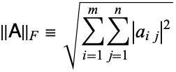
|| ||F는 Frobenius norm이라고 해서

이걸 의미하고, Tr은 trace of a matrix라고 한다.

 

 

이렇게 H와 Ar을 준비하고...

Diagonal 부분을 제거한 Ar을 Row normalize된 형태로 준비 한뒤... (However, we notice that A 𝑟 is a diagonal-dominant matrix, describing a graph with self-loops much stronger than any other connection. As self-loops usually hamper the propagation across adjacent nodes in message passing, 즉 message passing을 할때 self loop를 가장 많이 발생시키므로 제외했다고 한다.)

기본적으로 2 layer gcn이랑 동일하다.

 

이후

𝜃 is a dense layer for dimension conversion from 𝐶 ′ to 𝐶.

--> In practice, the matrix multiplication procedures for projection and reverse projection are both implemented by an 1×1 convolution layer since it supports high-speed parallelization.

 

 

 

 

In the meta learner, the two fully-connected layers have 𝑙𝑑 = 32 and 𝑙 𝑓 = 25 hidden units respectively and the embedding length 𝐷 is 64.